Bilinear Interpolation and Sparse Satellite Tracks

In my current work on data assimilation, the task involves querying satellite altimetry tracks for a given geospatial region and feeding them into a machine learning model. Given the curved grid that we have interpolated these tracks on, a geospatial query will retrieve a patch that is not exactly the desired patch sizes of ML ready inputs. Therefore, we need to resize/interpolate them as part of the data retrieval pipeline. However, I had blindly applied the standard PyTorch bilinear interpolation that is commonly used for standard images which causes a nice silent bug in the data pipeline.

The Setup

The particular tracks come from satellite altimetry that measure sea surface height. Unlike a standard RGB imagery or a dense grid of weather data, these observations are inherently sparse. A typical retrieved region might be 180×150 pixels, but only a thin set of near-vertical tracks actually contain valid measurements. The rest is NaN, no data. Coverage might just be 5–10% of the full patch size.

However, oftentimes ML pipeline need fixed-size inputs (say, 128×128), so at some point the retrieved geospatial patch has to be resized. The default approach in the Computer Vision domain is to use PyTorch’s F.interpolate with mode="bilinear" , which is commonly seen in every deep learning code base.

The Failure: Simple Bilinear Interpolation on raw sparse data

After noticing the issue, that the interpolation was removing much if not all of the original sparse tracks, I wanted to understand the issue in more detail. Bilinear interpolation computes a weighted average of the four nearest source pixels for every output pixel. That works beautifully when all four neighbors contain valid data. But when most of the grid is NaN, the arithmetic falls apart immediately.

Any operation involving NaN produces NaN. So if even one of the four neighbors is NaN (which, in a 5% coverage field, is almost guaranteed) the output pixel becomes NaN, meaning that the bilinear resize of sparse track data returns an almost entirely empty grid. Coverage drops from a modest but usable percentage to effectively zero. Your model receives a observation with no data.

Nearest Neighbor: A simple fix

The simplest fix is mode="nearest". Nearest-neighbor interpolation just copies the value of the single closest source pixel, no averaging, no neighbor mixing. Since it never combines pixels, a NaN stays a NaN and a valid value stays valid. Coverage is preserved.

The downside however is that the output can look blocky. There’s no smoothing, and the spatial structure has these staircase artifacts. So are there other approaches? Together with Claude I went down a little rabbit hole.

Sparse Resize: Mask-Weighted Bilinear Interpolation

So what are other possible alternativves? One idea is: what if we could do bilinear interpolation, but only over the valid pixels, while accounting for the sparse tracks explicitly?

The approach works in two parallel streams:

1. Zero-fill the data. Replace all NaNs with zero, then apply standard bilinear interpolation. This gives you a smooth but diluted result — wherever data was missing, the zeros drag the average down.

2. Interpolate a validity mask. Create a binary mask (1 where data exists, 0 where NaN), and bilinear-interpolate that mask with the same parameters. This mask tells you, for each output pixel, what fraction of its interpolation neighborhood was actually valid.

3. Divide. The ratio of the interpolated data to the interpolated mask undoes the dilution. If an output pixel’s neighborhood was only 30% valid, dividing by 0.3 rescales the average back to the correct magnitude. Where the mask is near zero (meaning essentially no valid neighbors), we set the output back to NaN.

def sparse_resize(data, size, mode="bilinear"):
    mask = torch.isfinite(data).float()
    data_zeroed = torch.nan_to_num(data, nan=0.0)

    data_resized = F.interpolate(data_zeroed, size=size, mode=mode, align_corners=False)
    mask_resized = F.interpolate(mask, size=size, mode=mode, align_corners=False)

    output = data_resized / (mask_resized + 1e-8)
    output[mask_resized < 1e-4] = float("nan")
    return output

This is elegant because it reuses the exact same bilinear kernel with the same smooth interpolation behavior, but the mask normalization ensures that the magnitude of the signal is preserved regardless of local data density. Tracks don’t bleed away into nothing. The coverage in the output closely tracks the coverage in the input, just remapped to the target grid.

Also note that we are interested in keeping track of the NaN areas before the data becomes a model input, because we need data availability as a mask.

Adaptive NaN Pool: Downsample by Averaging What’s There

The adaptive pooling approach is conceptually similar but uses a different geometric operation. Instead of bilinear interpolation (which maps each output pixel to a specific source location and blends neighbors), F.adaptive_avg_pool2d divides the source grid into bins corresponding to each output pixel and averages the bin contents.

The same mask trick applies:

def adaptive_nan_pool(data, output_size):
    mask = torch.isfinite(data).float()
    data_zeroed = torch.nan_to_num(data, nan=0.0)

    data_pooled = F.adaptive_avg_pool2d(data_zeroed, output_size)
    mask_pooled = F.adaptive_avg_pool2d(mask, output_size)

    output = data_pooled / (mask_pooled + 1e-8)
    output[mask_pooled < 0.05] = float("nan")
    return output

The pooling variant has a slightly different character. Because it averages over rectangular bins rather than using a smooth interpolation kernel, it can be better at consolidating scattered valid pixels within each bin. The 0.05 threshold on the mask is more permissive than the 1e-4 used in sparse resize it allows output pixels where at least 5% of the bin was valid, which can recover a bit more coverage in extremely sparse regions.

In practice, the two mask-weighted methods produce similar results. The choice between them often comes down to whether you’re upsampling (where bilinear makes more sense) or downsampling (where pooling is more natural).

A Note on Coverage

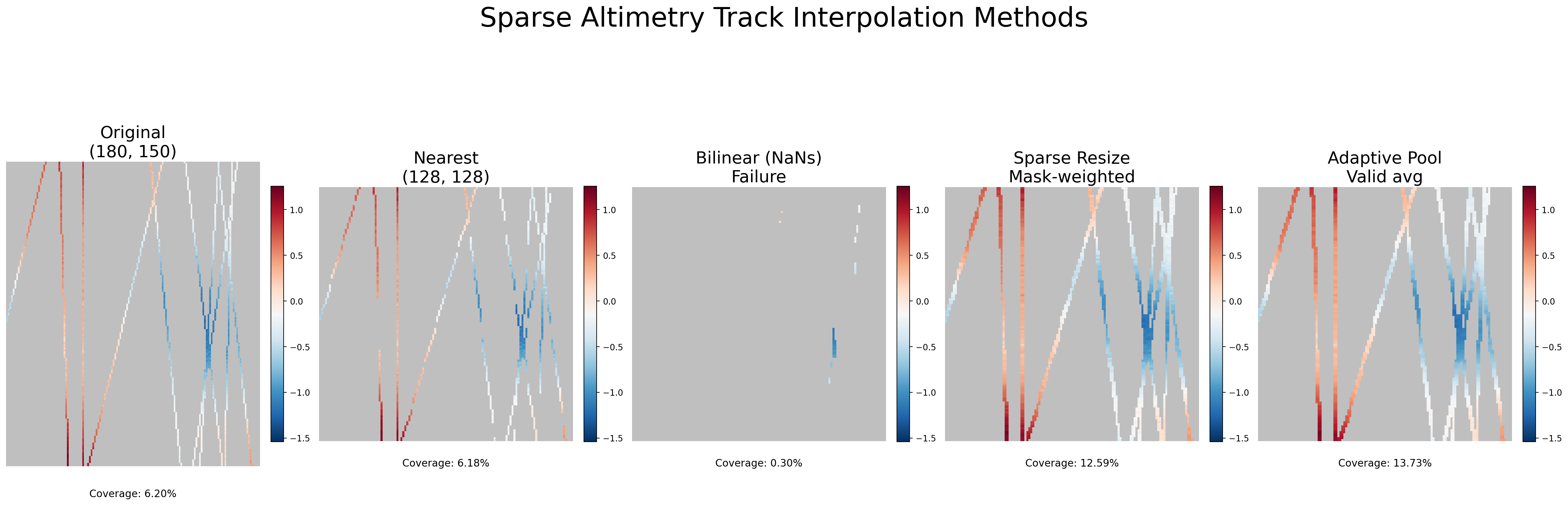
Looking at the comparison plot, one thing stands out: the mask-weighted methods don’t just preserve coverage, they actually increase it. The original data sits at 6.20% coverage, and nearest-neighbor faithfully preserves that at 6.18%. But sparse resize jumps to 12.59% and adaptive pooling to 13.73%.

This makes sense once you think about what each method is doing geometrically. In sparse resize, the bilinear kernel blends across a small neighborhood, so an output pixel can become valid even if only some of its four neighbors held data, as long as the interpolated mask exceeds the 1e-4 threshold. The interpolation effectively smears the tracks slightly wider than they were in the original. Similarly, adaptive pooling groups source pixels into rectangular bins, and any bin containing at least 5% valid pixels produces a valid output. Since a bin can span several source columns, a track that was one pixel wide in the source might contribute valid data to a wider footprint in the output.

In both cases, the mask-and-divide approach is more permissive than the original binary valid/invalid distinction, it recovers partial information from mixed neighborhoods. Nearest-neighbor, by contrast, does a strict one-to-one copy, so coverage stays almost identical (the tiny 0.02% drop is just rounding from the grid remapping).

Whether this extra coverage is desirable depends on the use case. If you want to preserve exactly the spatial footprint of the original observations, nearest-neighbor is more faithful. If you’re okay with mild spatial smoothing in exchange for denser inputs to your model, the mask-weighted methods give you that for free.

Conclusion

The fix here isn’t complicated, but this was a classic silent bug, where the pipeline runs smoothly but carrying a severe bug. The failure mode is insidious precisely because bilinear interpolation is so universally used.

Sparse geospatial observations such as altimetry tracks or scattered in-situ measurements break that assumption quietly. No error is raised, the tensor has the right shape, and the pipeline runs.

If you want to play around with this yourself, I made a small self-contained script that generated the above figure. It is available in this gist.